Single Screw Performance Characterization
Vol. 31 #2, Fall 2004
Introduction
An extruder technician should understand the extruder performance characteristics. Performance characteristics describe the equipment behavior. To use a medical analogy, performance characteristics are like a treadmill test report. The patient is put through their paces and his/her performance is recorded. When we characterize an extruder or any equipment, we put it through its operating range to determine its performance. With this information, we have a reference point from which we can compare future behavior and diagnose equipment problems.
The doctor uses physical exams to establish a performance baseline. If the patient gets sick, the doctor’s job is to diagnose the disease and prescribe a remedy. This section describes how to give the extruder a physical and to characterize its performance. There are two basic characteristics to explore: extruder output and control sensitivity. The first characteristic to understand is the extruder’s output as a function of RPM. The second is the control sensitivity of variables such as zone temperature at an RPM close to that expected during normal operation.
In looking at the extruder’s output as a function of RPM the following graphs are useful.
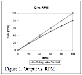
Figure 1, output vs. RPM, shows the actual screw performance vs. the drag flow or the screw designer’s calculation. In most cases, backwards pressure flow lowers the actual output below the drag flow because of the increasing pressure profile in most extrusion systems. In some cases, such as when an extruder is designed with a cooled grooved feed throat, the output can be higher than the drag flow calculation. Other designs cause a pressure peak before the metering section, and those designs will give outputs close to the drag flow calculation.
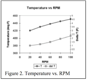
Figure 2, temperature and delta temperature vs. RPM, shows the melt temperature and temperature variability. Temperature variability is difficult to measure. The design of your thermocouple and its radial positioning in the melt stream are important variables in measurements of the actual temperature variations. Exposed junction thermocouples placed about one third of the way into the melt stream will give the most sensitive and accurate measurements. Shielded thermocouples placed at the melt pipe wall give the poorest response and may measure only the melt pipe temperature. Steward (2) recommends using the following equation to calculate the minimum immersion depth for an exposed junction thermocouple in order to measure accurate temperatures.
Dmin (inch) = (0.3 + Bore Diam (inch) - 0.75) / 5
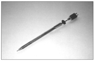
Above is a picture of an exposed junction adjustable depth melt thermocouple. One rotates the thumb wheel between the thermocouple barrel and the thermocouple connector to adjust the immersion depth. These thermocouples can be damaged if unmelted polymer is pushed past the protruding measuring junction. To avoid damage:
- Allow sufficient time for complete melting before allowing the screw to turn in a cold extruder or
- Retract the probe when shutting down the extruder and then reposition it in the melt stream after flow is established.
For accurate temperature measurements, the following observation by Steward (3) gives a qualitative correlation with melt quality or uniformity.
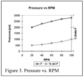
Figure 3, pressure and percent pressure fluctuations vs. RPM, shows how much pressure is required to pump poly- mer through your downstream filter, piping and die. The pressure fluctuation measures your extrusion system’s stability. If the head pressure (measured downstream of the last flight) is stable, then flow is stable. For non-Newtonian fluids (such as polymers) that follow the power law, flow variation is a function of pressure variation and can be calculated. In extrusion, one can predict the change in out- put resulting from a change in pressure or temperature. It can be shown that the relationship between output and pressure change is approximately (4):
dQ (%) = dP (%) / n
Where:
dQ (%) = Percent change in flow rate
dP (%) = Percent change in head pressure
n = Power law index of melt at given shear rate and temperature.
As an example, for polypropylene with a power law index of n = 0.35, a 3% total variation in pressure will cause an 8.6% variation in output. For a shear thinning plastic melt, the out- put change will always be larger than the pressure change (5). The following table contains representative power law indexes for several plastics.
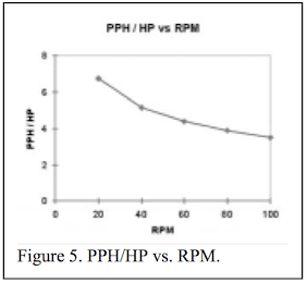
Figures 4 and 5 are measures of screw efficiency. Figure 4, pounds per hour vs. RPM, is really the slope or first derivative of the rate curve vs. RPM. The greater the negative slope of this graph, the poorer the screw efficiency at higher RPM. Figure 5 shows the energy efficiency and the conversion of motor power to melt temperature and pressure. This curve is an excellent way to measure performance vs. time and to compare alternate screw designs.
Once a performance baseline is established, then one can look at operating variables and determine which variables can improve the process and which variables are not significant. An efficient way to do this is with a statistically designed experiment. There are many experimental designs and different combinations of independent variables combinations to choose from. It is important that a team pools their knowledge under the guidance of a trained statistician to model the process, utilizing sequential experimental design (SED), or as alternatively known, design of experiments (DOE). SED is organized into three phases. The first phase is for screening. This phase requires 25% of the required resources and uses fractional factorial (FF) techniques. The second phase uses 50%-60% of the resources and utilizes central composite designs (CCD) to build a process model. The third R phase, verification uses 15%-25% of the resources and takes advantage of simulation or “Taguchi” techniques (6).
- John R. Wagner, Jr., Crescent Associates, Inc.
References1. J.R. Wagner, Jr., “Screw Characterization” Calhoun, A., Wagner, Jr., J.R. Editors SPE Plastics Technician’s Toolbox® – Extrusion, Society of Plastics Engineers (2004).
2. E. Steward, “Melt Temperature Considerations for Extrusion – Presentation Slides,” SPE ANTEC, 46, 364 (2000).
3. E. Steward, “Melt Temperature Considerations for Extrusion,” SPE ANTEC, 46, 364 (2000).
4. J.R. Wagner, Jr., Output variation 1, SPE Extrusion Division Extrusion Solutions CD ver.1.0 (2000).
5. C. Rauwendaal, “The Effect of Pressure on Output,” SPE Extrusion Division Newsletter, Vol. 17, No. 3 (December 1990).
6. T.B. Barker, Quality by Experimental Design, 2nd Edition, p. 24, Marcel Dekker (1994).
Return to
Consultants' Corner